Exponential Distribution
Introduction
This is a short reminder of some simple properties of exponential distributions.
The continuous random variable (RV) \(\xi\) has an exponential distribution with the rate \(\lambda>0\) if its CMD (cumulative distribution function) has the following form
\[F_\xi(x)=P(\xi<x)=\left\{\begin{matrix} &1-e^{-\lambda x}, &x\geq 0.\\ &0 &x<0. \end{matrix}\right. \] This entails that an exponential RV is with 1 probability positive and has the PDF (probability density function) \[f_\xi(x)=F_\xi'(x)=\left\{\begin{matrix} &\lambda e^{-\lambda x}, &x>0,\\ &0 &x<0. \end{matrix}\right. \] If \(\xi\) has an exponential distribution with the rate \(\lambda\) we will denote this by \({\mathbb E}(\lambda).\)
In \(R\) the following functions can be used to, correspondingly, generate numbers from \({\mathbb E}(\lambda)\), calculate values of CDF, calculate values of PDF
rexp(n=2, rate=1)## [1] 2.769818 1.201461pexp(q=1, rate=1)## [1] 0.6321206dexp(x=1, rate=1)## [1] 0.3678794The histogram is a non-parametric estimator for the PDF. Hence we can simulate data from an exponential distribution and show that the histogram based on the data fits the PDF. Consider the case of \({\mathbb E}(2)\) and simulate a sample of size \(n=10000.\)
rm(list=ls())

n <- 10000
lambda <- 2

X <- rexp(n = n, rate = lambda)
int <- seq(0, max(X), max(X)/100)

hist(X, freq = FALSE, nclass = 50, col = "lightblue",
     border = "blue", ylim = c(0, 2), main = "")
lines(int, dexp(int, rate = lambda), col = "red", lty = 2, lwd = 2)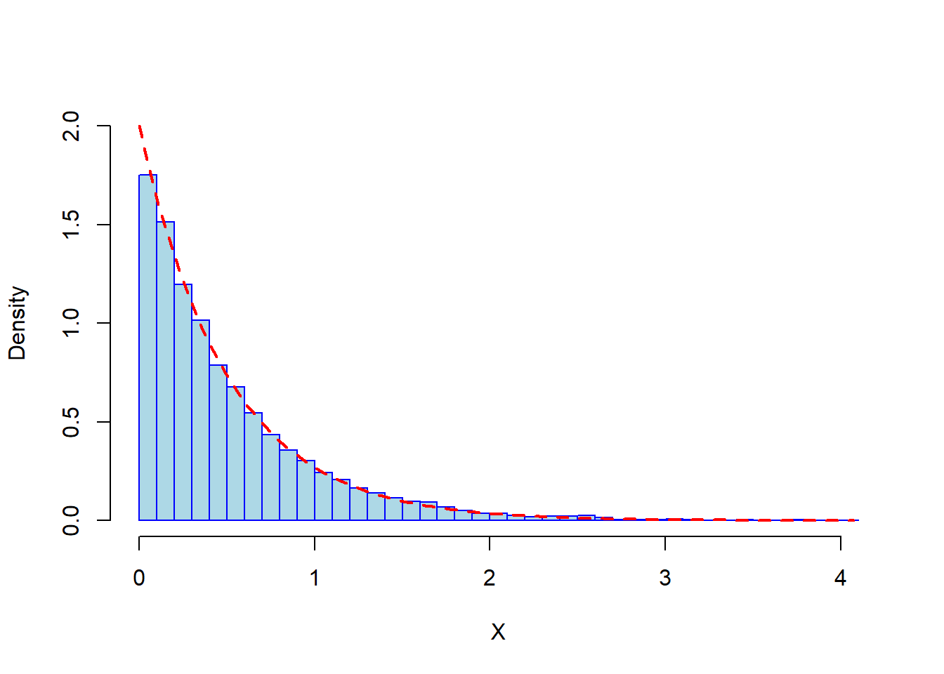
This is a very useful technique to check whether the RVs have the given PDF. We will use this technique below.
Example 1
Suppose \(\xi\sim {\mathbb E}(\lambda)\) and \(\eta\sim {\mathbb E}(\mu)\) are independent. Calculate the PDF of the RV \(\zeta=\eta-\xi.\)
First consider the case of \(z>0.\) Since \(\xi\) and \(\eta\) are independent, then the joint PDF of these RVs will be the product of individual PDFs, that is \(f_{(\eta,\xi)}(x,y)=f_{\xi}(x)f_{\eta}(y).\) Therefore,
\[F_\zeta(z)=P(\eta-\xi<z)=\int_0^{+\infty}\int_0^{+\infty}I_{\{y-x\leq z\}}(x,y)\lambda\mu e^{-\lambda x-\mu y}d x dy.\] Making the following variable change \(u=y-x\) will give \[F_\zeta(z)=P(\eta-\xi<z)=\lambda\mu \int_0^{+\infty}e^{-(\lambda + \mu) x}\left(\int_{-x}^{z}e^{-\mu u}d u\right) dx=1-\frac{\lambda}{\lambda+\mu}e^{-\mu z},\ \ z>0.\] If \(z<0\) then \[P(\eta-\xi<z)=P(\xi-\eta>-z)=1-P(\xi-\eta<-z)=1-\left(1-\frac{\mu}{\mu+\lambda}e^{\lambda z}\right)=\frac{\mu}{\lambda+\mu}e^{\lambda z},\ \ z<0.\] Therefore, \[F_\zeta(z)=\left\{\begin{matrix} &1-\frac{\lambda}{\lambda+\mu} e^{-\mu z}, &z\geq 0,\\ &\frac{\mu}{\lambda+\mu} e^{\lambda z} &z<0. \end{matrix}\right.\] The PDF will be \[f_\zeta(z)=\frac{\lambda\mu}{\lambda+\mu}\left\{\begin{matrix} &e^{-\mu z}, &z\geq 0,\\ &e^{\lambda z} &z<0. \end{matrix}\right.\] This formula can be checked using simulations.
rm(list=ls())

n <- 20000
m <- 10000
lambda <- 2
mu <- 5


  X <- rexp(n,lambda)
  Y <- rexp(m, mu)
  Z <- Y-X

int <- seq(min(Z),max(Z),(max(Z)-min(Z))/100)
dens <- function(z) (lambda*mu)/(lambda+mu)*ifelse(z>=0,exp(-mu*z),exp(lambda*z))
hist(Z, nclass = 100, freq=FALSE,ylim=c(0,1.5),
     xlim = c(min(Z),max(Z)), main="", col = "lightblue", border = "blue")
lines(int,dens(int), col="2")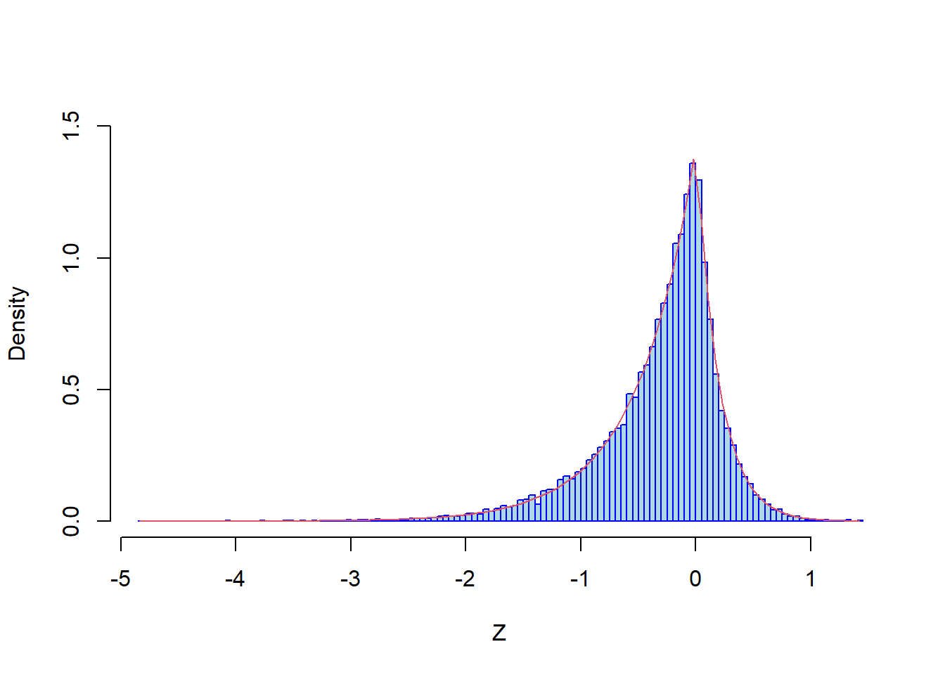
From the PDF we can calculate also \[E(\zeta)=\frac{\lambda-\mu}{\lambda\mu},\ \ P(\eta>\xi)=\frac{\lambda}{\lambda+\mu}.\]
Example 2
Suppose that \(\eta\sim{\mathbb E}(\mu)\) and \(\eta'\sim{\mathbb E}(\mu')\) are independent. Find the distribution of the RVs \(\min(\eta,\eta')\) and \(\max(\eta,\eta').\)
For all \(z>0\) we have \[\begin{align*} P(\min(\eta,\eta')<z)=1-P(\min(\eta,\eta')\geq z)=1-P(\eta\geq z,\eta'\geq z)=1-e^{-(\mu+\mu') z},\,z>0, \end{align*}\] and \(P(\min(\eta,\eta')<z)=0,\ \ z\leq 0.\) Therefore, \(\min(\eta,\eta')\sim{\mathbb E}(\mu+\mu')\), that is, the minimum of two exponentially distributed RVs is an exponentially distributed RV as well, with the rate being equal to the sum of the rates of the given two RVs.
On the other hand, \[P(\max(\eta, \eta') < z)= P(\eta < z, \eta' <z)=(1-e^{-\mu z})(1-e^{-\mu' z}),\,z>0.\] For \(\mu=\mu'\) we have
\[P(\max(\eta, \eta') < z) = (1-e^{-\mu z})^2,\,z>0,\] with PDF being equal to \(f(z)=2\mu(1-e^{-\mu z})e^{-\mu z},\,z>0\) and \(f(z)=0,\,z<0.\)
Example 3
For given three independent RVs such that \(\xi\sim{\mathbb E}(\lambda)\) and \(\eta,\eta'\sim{\mathbb E}(\mu),\) calculate the following probability \(\theta=P(\xi<\eta,\xi<\eta').\)
We can reformulate this problem as follows \[\theta=P(\xi<\eta,\xi<\eta')=P(\xi<\min(\eta,\eta'))=P(\xi-\min(\eta,\eta')<0).\] Hence, denoting by \(\zeta=\xi-\min(\eta,\eta'),\) in the first step we can calculate the distribution function of the RV \(\zeta.\) We have \(\xi\sim{\mathbb E}(\xi)\) and \(\min(\eta,\eta')\sim{\mathbb E}(2\mu)\) (see Example 2), hence, using the Example 1 we obtain
\[F_\zeta(z)=\left\{\begin{matrix} &1-\frac{2\mu}{\lambda+2\mu} e^{-\lambda z}, &z\geq 0,\\ &\frac{\lambda}{\lambda+2\mu} e^{2\mu z} &z<0. \end{matrix}\right.\] For the PDF we have \[f_\zeta(z)=\left\{\begin{matrix} &\frac{2\lambda\mu}{\lambda+2\mu} e^{-\lambda z}, &z> 0,\\ &\frac{2\lambda\mu}{\lambda+2\mu} e^{2\mu z} &z<0. \end{matrix}\right.\] We can, again, check this using simulations.
rm(list=ls())

n <- 200000
m <- 100000
lambda <- 2.5
mu <- 1.3


X1 <- rexp(n,mu)
X2 <- rexp(n,mu)
Y <- rexp(m, lambda)
Z <- Y - ifelse(X1>=X2,X2,X1)
Coeff <- 2*lambda*mu/(lambda+2*mu)

int <- seq(min(Z), max(Z), (max(Z)-min(Z))/100)
dens <- function(z) Coeff*ifelse(z>=0, exp(-lambda*z), exp(2*mu*z))


hist(Z, nclass = 100, freq=FALSE, ylim=c(0,1.5),
     xlim=c(min(Z), max(Z)), main = "", border = "blue", col = "lightblue")
lines(int,dens(int), col="2")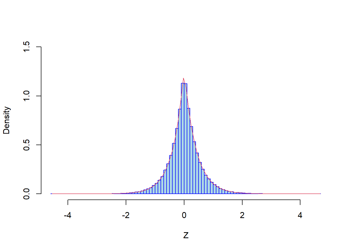
Therefore, \[\theta=F_\zeta(0)=\frac{\lambda}{\lambda+2\mu}.\]
Example 4
For given three independent RVs such that \(\xi,\xi'\sim{\mathbb E}(\lambda)\) and \(\eta\sim{\mathbb E}(\mu),\) calculate the following probability \(\vartheta=P(\xi<\eta,\xi'<\eta).\)
We can reformulate this problem as follows \[\vartheta=P(\xi<\eta,\xi'<\eta)=P(\max(\xi,\xi')<\eta)=P(\eta-\max(\xi,\xi')>0).\] Hence, denoting by \(\kappa=\eta-\max(\xi,\xi'),\) in the first step we can calculate the distribution function of the RV \(\kappa.\)
\[\begin{align*} P(\kappa<z)=\int_0^{+\infty}\int_0^{+\infty}I(y-x\leq z)2\lambda\mu(1-e^{-\lambda x})e^{-\lambda x-\mu y}d x d y. \end{align*}\] If \(z>0\) then, denoting \(y-x=u\) we get \(y=u+x,\,u\in[-x,\infty)\ \ d y= d u.\) Therefore,
\[\begin{align*} P(\kappa<z)&=2\lambda\mu\int_0^{+\infty}(1-e^{-\lambda x})e^{-\lambda x-\mu x}\int_{-x}^{z}e^{-\mu u}d u d x=\\ &=-2\lambda\int_0^{+\infty}(e^{-(\lambda+\mu) x -\mu z}-e^{-(2\lambda+\mu) x -\mu z}-e^{-\lambda x }+e^{-2\lambda x }) d x=\\ &=1-\frac{2\lambda^2}{(\lambda+\mu)(2\lambda+\mu)}e^{-\mu z },\ \ z>0. \end{align*}\] For \(z>0\) calculate also (using the notation \(x-y=u\), which entails \(x=y+u,\,d x=d u,\) where \(u\in[-y,+\infty).\)) \[\begin{align*} P(\max(\xi,\xi')-\eta<z)&=\int_0^{+\infty}\int_0^{+\infty}I(x-y\leq z)2\lambda\mu(1-e^{-\lambda x})e^{-\lambda x-\mu y}d x d y=\\ &=\int_0^{+\infty}\int_{-y}^{z}(e^{-\lambda(y+u) - \mu y} - e^{-2\lambda(y+u) -\mu y}d u dy)=\\ &=1+\mu\left[\frac{e^{-2\lambda z}}{2\lambda+\mu}-\frac{2e^{-\lambda z}}{\lambda+\mu}\right],\ \ z\geq 0. \end{align*}\]
Therefore, for \(z>0\) we have \[\begin{align*} P(\kappa<-z)&=1-P(\max(\xi,\xi')-\eta<z)=\\ &=-\mu\left[\frac{e^{-2\lambda z}}{2\lambda+\mu}-\frac{2e^{-\lambda z}}{\lambda+\mu}\right],\ \ z\geq 0 \end{align*}\] Finally we obtain \[F_\kappa(z)=\left\{\begin{matrix} &1-\frac{2\lambda^2}{(\lambda+\mu)(2\lambda+\mu)} e^{-\mu z}, &z\geq 0,\\ &-\mu\left[\frac{e^{2\lambda z}}{2\lambda+\mu}-\frac{2e^{\lambda z}}{\lambda+\mu}\right] &z<0. \end{matrix}\right.\] For the PDF we have \[f_\kappa(z)=\left\{\begin{matrix} &\frac{2\lambda^2\mu}{(\lambda+\mu)(2\lambda+\mu)} e^{-\mu z}, &z> 0,\\ &-2\lambda\mu\left[\frac{e^{2\lambda z}}{2\lambda+\mu}-\frac{e^{\lambda z}}{\lambda+\mu}\right] &z<0. \end{matrix}\right.\] To check this formula we can make the following simulations.
rm(list=ls())

n <- 200000
m <- 100000
lambda <- 2.5
mu <- 5.5


X1 <- rexp(n,lambda)
X2 <- rexp(n,lambda)
Y <- rexp(m, mu)
Z <- Y - ifelse(X1 >= X2, X1, X2)
Coeff <- 2*mu*lambda^2/((lambda+mu)*(2*lambda+mu))
Coeff1 <- -2*lambda*mu/(2*lambda+mu)
Coeff2 <- -2*lambda*mu/(lambda+mu)

int <- seq(min(Z), max(Z), (max(Z)-min(Z))/100)

dens <- function(z) ifelse(z>=0, Coeff*exp(-mu*z),
                           Coeff1*exp(2*lambda*z)-Coeff2*exp(lambda*z))


hist(Z, nclass = 100, freq=FALSE,ylim=c(0, 1.5), xlim=c(min(Z), max(Z)),
     main = "", col = "lightblue", border = "blue")
lines(int,dens(int), col="2")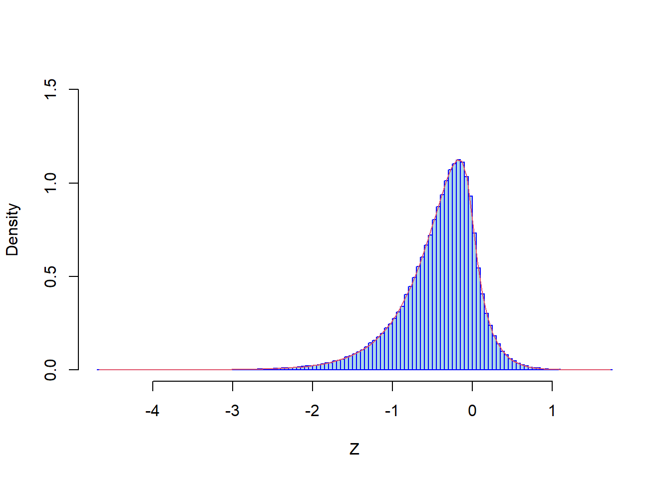
Therefore, \[\vartheta=P(\xi<\eta, \xi'<\eta)=P(\kappa>0)=\frac{2\lambda^2}{(\lambda+\mu)(2\lambda+\mu)}.\]