Introduction

Hierarchical composite endpoints (HCE) are complex endpoints combining events of different clinical importance into an ordinal outcome that prioritize the most severe event of a patient. Up to now, one of the difficulties in interpreting HCEs has been the lack of proper tools for visualizing the treatment effect captured by HCE. This package makes it possible to visualize endpoints consisting of the combination of one to several time-to-event (TTE) outcomes (like Death, Hospitalization for heart failure, …) with one continuous outcome (like a symptom score).

The maraca plot (introduced in (Martin Karpefors, Lindholm Daniel, and Samvel B. Gasparyan 2022)) captures all important features of how the HCE measures the treatment effect: 1. the percentage of time-to-event outcomes in the overall population, 2. the treatment effect on the combined and individual time-to-event outcomes, and 3. the treatment effect on the continuous component.

Basic usage

Plotting with maraca package (Martin Karpefors and Samvel B. Gasparyan 2022) requires to have the data in an appropriate format. We provide a few scenarios in the package, named hce_scenario_a, hce_scenario_b, hce_scenario_c and hce_scenario_d. These scenarios cover four cases: a) Treatment effect is driven by a combination of TTE outcomes and continuous outcome, b) No treatment effect on neither the TTE outcomes nor on the continuous outcome, c) A large treatment effect on time-to-event outcomes, but no effect on continuous outcome, and finally d) A small treatment effect on time-to-event outcomes, with a larger effect on continuous outcomes, respectively. Other HCE scenarios can easily be simulated with the hce package (Gasparyan 2022). The hce package is also used for win odds calculations in the maraca package.

library(maraca)

data(hce_scenario_a, package = "maraca")

data <- hce_scenario_a
head(data)
##   X SUBJID              GROUP GROUPN      AVAL0       AVAL    TRTP
## 1 1      1          Outcome I      0 120.440921   120.4409  Active
## 2 2      2 Continuous outcome  40000   3.345229 40003.3452 Control
## 3 3      3 Continuous outcome  40000  22.802615 40022.8026  Active
## 4 4      4          Outcome I      0 577.311386   577.3114 Control
## 5 5      5         Outcome II  10000 781.758081 10781.7581  Active
## 6 6      6        Outcome III  20000 985.097981 20985.0980 Control

The data data frame contains information on various columns. These columns may have arbitrary names, so the maraca function allows you to specify these names and how they map to the internal nomenclature using the column_names parameter. This parameter is a named character vector, mapping the standard names used by maraca with the column names in your dataset.

column_names <- c(
    outcome = "GROUP",
    arm = "TRTP",
    value = "AVAL0"
)

the outcome column must be a character column containing the outcome for each entry.

unique(data[["GROUP"]])
## [1] "Outcome I"          "Continuous outcome" "Outcome II"        
## [4] "Outcome III"        "Outcome IV"

The strings associated to each entry are arbitrary, so maraca allows you to specify them in the tte_outcomes and continuous_outcome parameters. Make sure to specify the TTE outcomes in the correct order, starting from the most severe outcome to the least severe outcome. There can only be one continuous outcome.

tte_outcomes <- c(
  "Outcome I", "Outcome II", "Outcome III", "Outcome IV"
)
continuous_outcome <- "Continuous outcome"

the arm column must also be a character column describing to which arm each row belongs.

unique(data[["TRTP"]])
## [1] "Active"  "Control"

The strings associated to each entry are arbitrary, so maraca allows you to specify them in the arm_levels parameter, as a named vector of character strings. In this example, our file contains “Active” and “Control” as identifiers, as seen in the output above, so we will specify

arm_levels = c(active = "Active", control = "Control")

Finally, the original column must contain numerical values.

All of the above can be aggregated in the call to create a maraca object from the given dataset

mar <- maraca(
  data, tte_outcomes, continuous_outcome, arm_levels, column_names, compute_win_odds = TRUE
)

The win odds can be calculated and will be annotated in the maraca plot if available. However, it is not calculated by default. Please set the compute_win_odds = TRUE to make the calculation. The resulting estimate, 95% confidence levels and p-value will be shown in the maraca object and can also be retrieved with

mar$win_odds
##     estimate        lower        upper      p-value 
## 1.643265e+00 1.416117e+00 1.906848e+00 9.354073e-12

Plotting the resulting object

To create a maraca plot, simply pass the maraca object as the first argument to the plot function. In addition to the maraca object, the user can optionally supply input parameters for selecting the continuous_grid_spacing; transforming the x-axis using “sqrt” in the trans argument; selecting different representations of the continuous distribution density in the density_plot_type; and setting vline_type to “mean” or “median”.

The following types of plots that are available: “default”, “violin”, “box”, “scatter”. The default type is just a nested combination of violin and box plot. Figure 1A-D in reference 1 below, can be recreated through applying the maraca function with subsequent plotting on each of the scenario A-D datasets provided in this package. As an example scenario A is shown in the following plot.

plot(mar, continuous_grid_spacing_x = 20)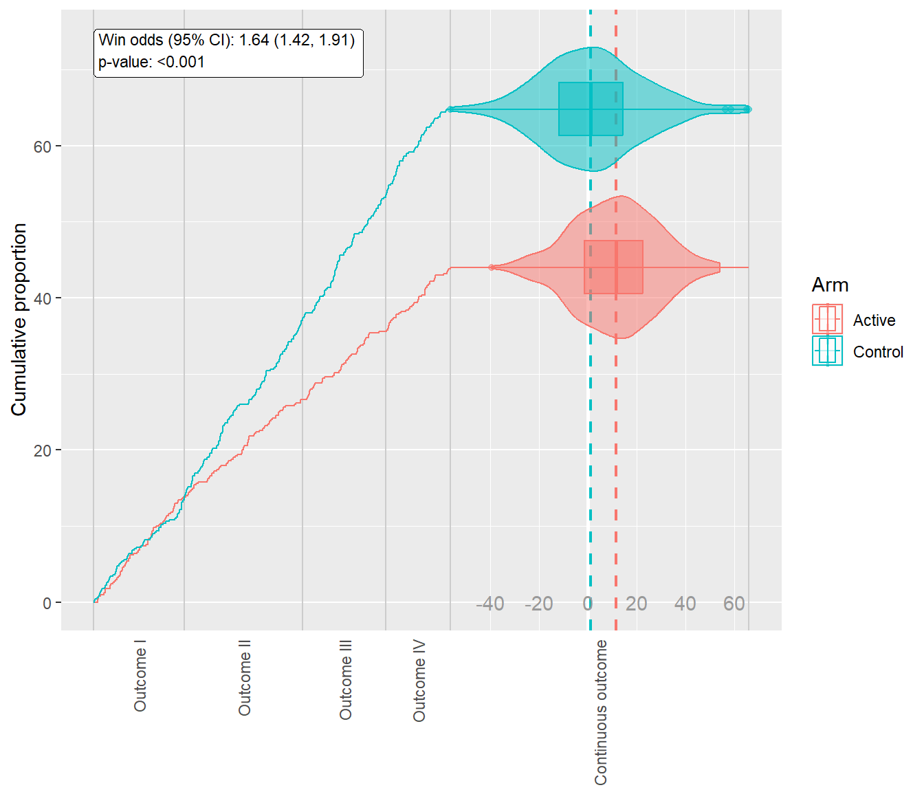

plot(mar, continuous_grid_spacing_x = 20, density_plot_type = "box")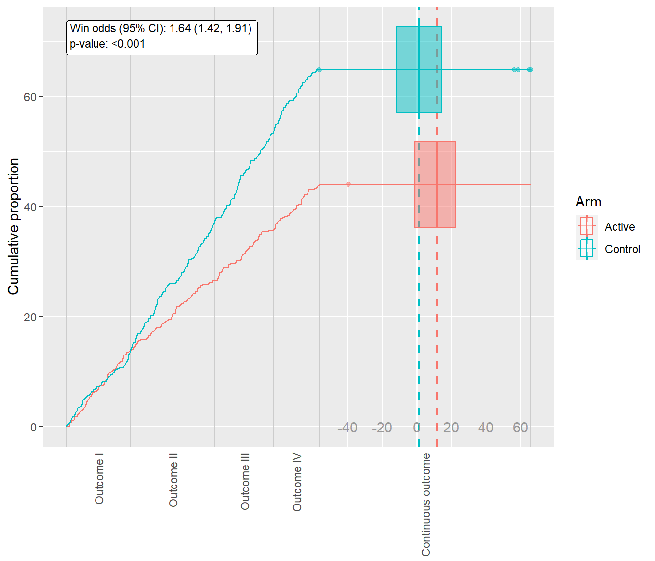

plot(mar, continuous_grid_spacing_x = 20, density_plot_type = "scatter", vline_type = "mean")
## Warning: Removed 1 rows containing missing values (`geom_point()`).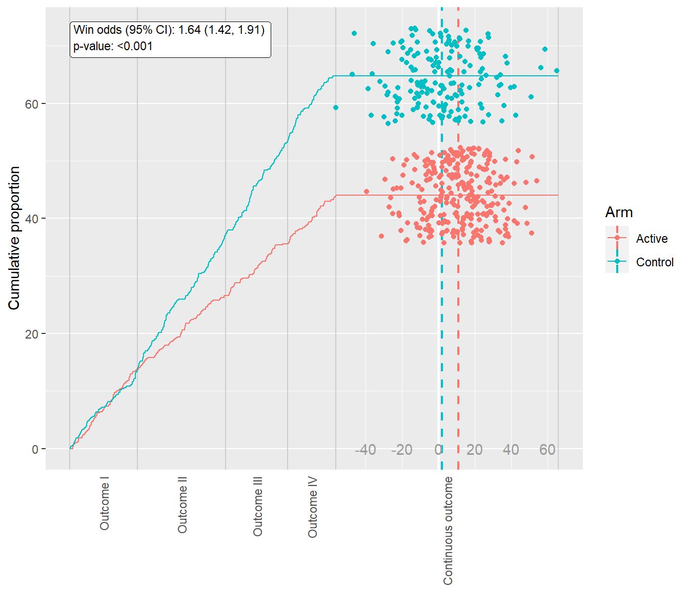

The plot_maraca function returns a ggplot2 object. This function will not render the plot immediately so you will have to print() it. Conveniently, you can customize your maraca plot with the comprehensive toolbox of ggplot2. For example:

p <- plot_maraca(mar, continuous_grid_spacing_x = 20, density_plot_type = "scatter", vline_type = "mean")
p + 
  theme_bw() + scale_color_manual(values=c("#999999", "#E69F00")) + 
  theme(axis.text.x.bottom = element_text(vjust = 0.5, hjust = 0.5))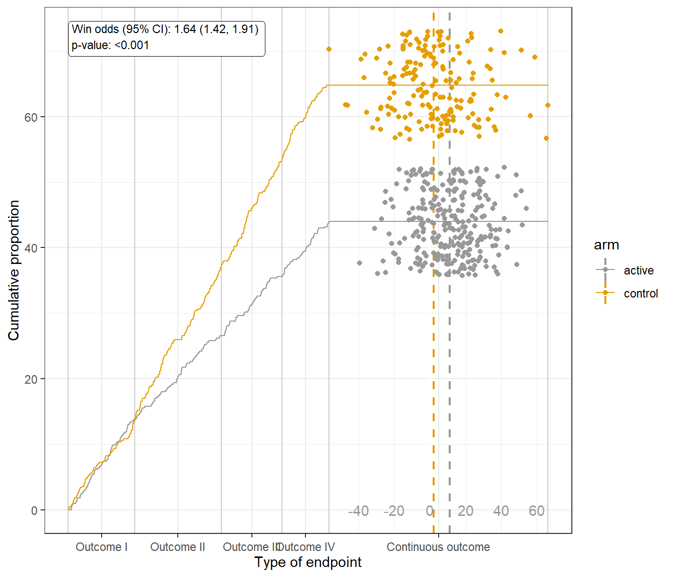

Additionally, there are a few supporting plots that can be used to look closer at the time-to-event outcomes. plot_tte_components provides a one-row grid of the TTE outcomes Kaplan-Meier plots.

plot_tte_components(mar)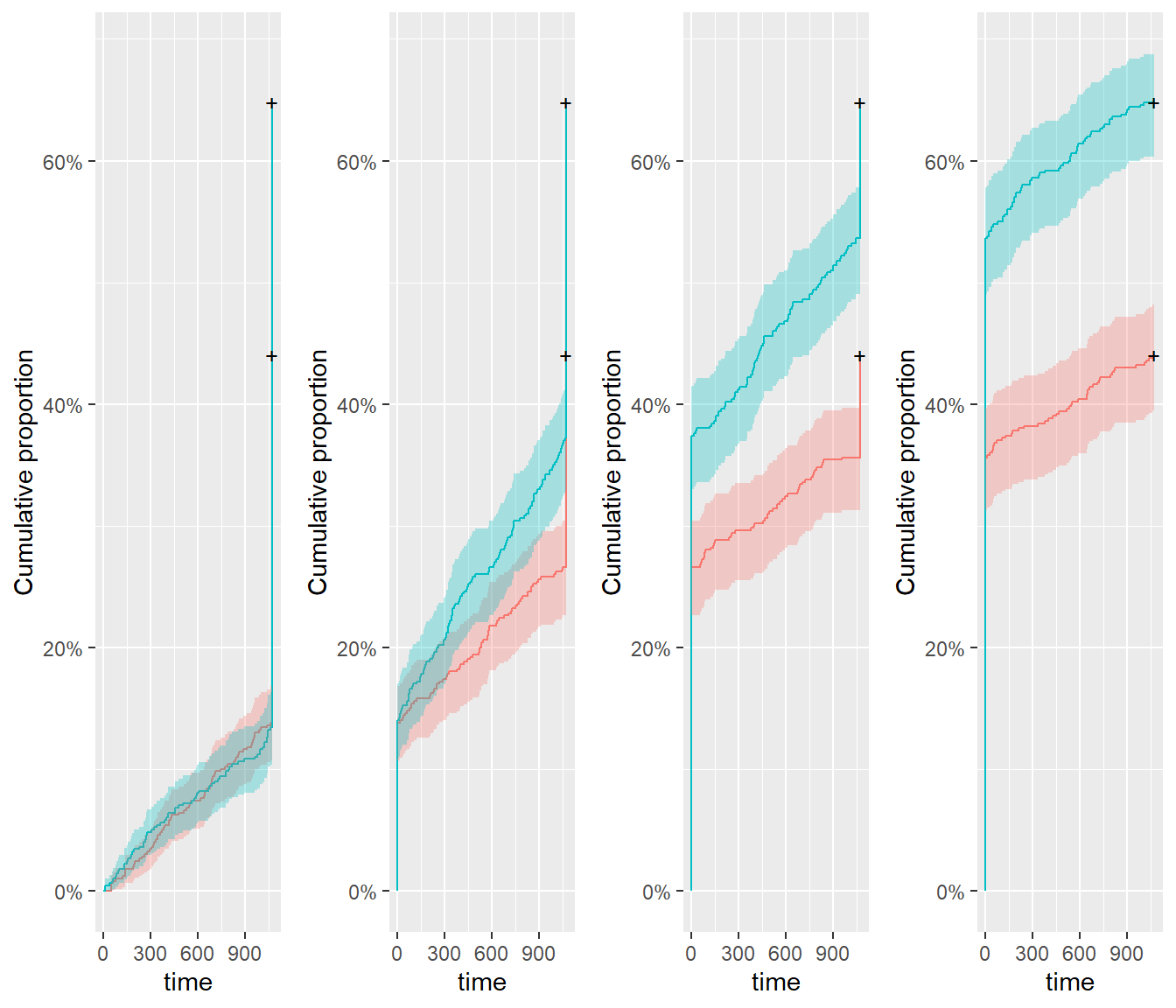

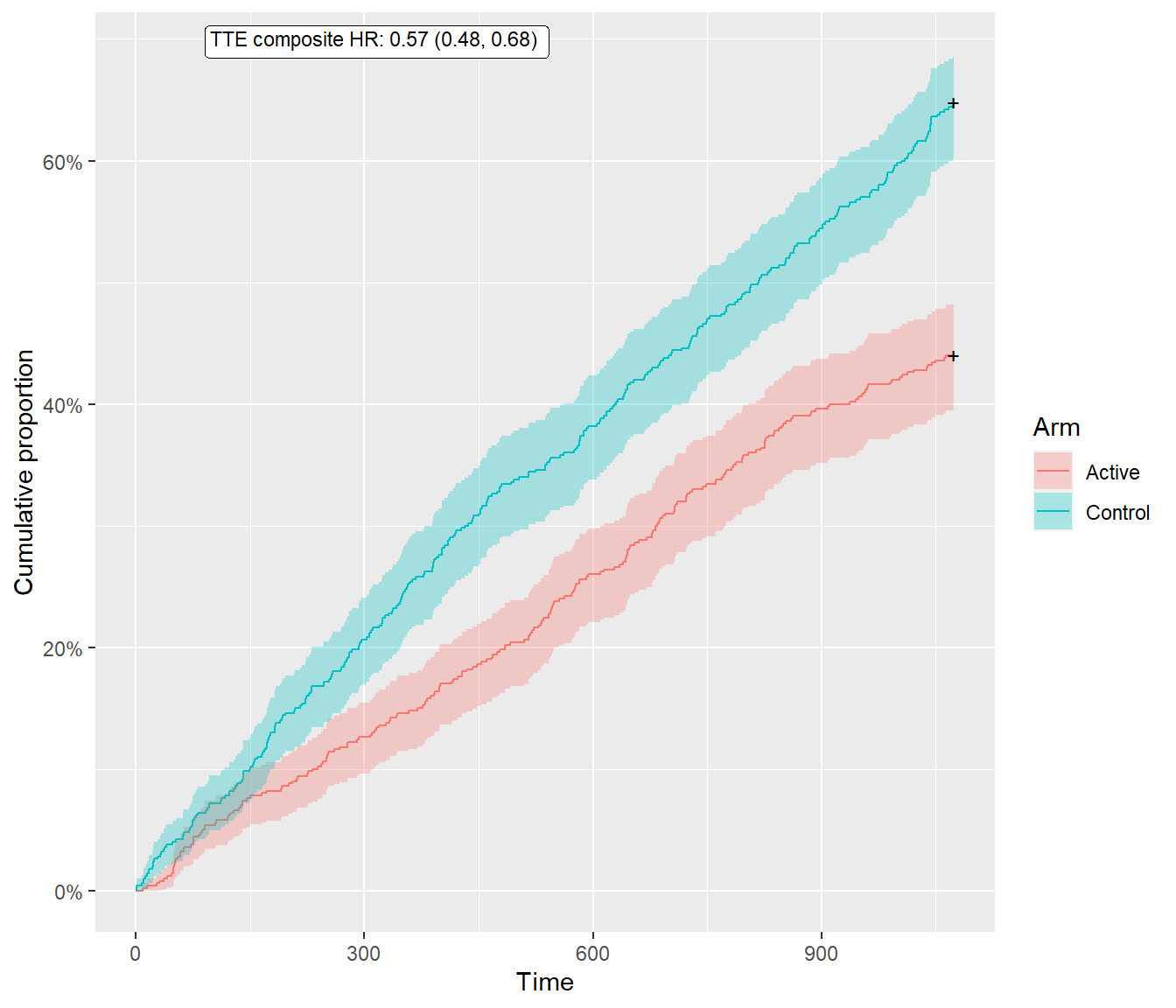
plot_tte_composite plots the Kaplan-Meier plot for the composite of all specified events. The plot is also annotated with the hazard ratio (more info in mar$survmod_complete).

plot_tte_composite(mar)