Win Odds Confidence Intervals in R

Mann-Whitney estimate for the win probability

Consider two independent, continuous RVs (random variables) \(\xi\) and \(\eta\). The following probability is called the win probability of RV \(\eta\) against the RV \(\xi\)

\[\begin{align*} \theta=P(\eta>\xi). \end{align*}\]

Given an i.i.d. (independent, identically distributed) random sample from \(\xi,\) denoted by \(X=(X_1,\cdots,X_{n_1})\) and an i.i.d. sample from \(\eta\) denoted by \(Y=(Y_1,\cdots,Y_{n_2})\) we are interested in estimating the unknown parameter \(\theta.\)

The following estimator is called the Mann-Whitney estimator (or, the win proportion) for the win probability

\[\begin{align*} \hat\theta_N=\frac{1}{n_1n_2}\sum_{i=1}^{n_1}\sum_{j=1}^{n_2}I(X_i<Y_j). \end{align*}\] Here \(N=n_1+n_2\) is the total sample size, whereas \(I(\cdot)\) is the indicator function which takes the value 1 if the underlying inequality is true and 0 otherwise. When \(n_1\rightarrow+\infty,\,n_2\rightarrow+\infty\) then the win proportion is a consistent estimator (convergence in probability) for the win probability \[\begin{align*} \hat\theta_N\longrightarrow\theta. \end{align*}\] If \(\frac{n_1}{N}\rightarrow \alpha,\) as \(n_1\rightarrow+\infty,\,n_2\rightarrow+\infty,\) then the win proportion is also asymptotically normal (Van der Vaart 2000) \[\begin{align*} \sqrt{N}(\hat\theta_N-\theta)\Longrightarrow{\mathcal N}\left(0,\frac{1}{1-\alpha}\sigma_{10}^2+\frac{1}{\alpha}\sigma_{01}^2\right). \end{align*}\] Here, \[\begin{align*} \sigma_{10}^2=Cov(I(\xi<\eta),I(\xi'<\eta))=P(\xi<\eta,\xi'<\eta)-P(\xi<\eta)^2,\\ \sigma_{01}^2=Cov(I(\xi<\eta),I(\xi<\eta'))=P(\xi<\eta,\xi<\eta')-P(\xi<\eta)^2, \end{align*}\] where \(\xi'\) has the same distribution as \(\xi\), \(\eta'\) has the same distribution as \(\eta\). All \(\xi,\xi',\eta,\eta'\) are independent.

Application to exponential distributions

Suppose now that \(\xi\sim{\mathbb E}(\lambda)\) and \(\eta\sim{\mathbb E}(\mu).\) In this case,

\[\begin{align*} \sigma_{10}^2=\frac{2\lambda}{(\lambda+\mu)(2\lambda+\mu)}-\frac{\lambda^2}{(\lambda+\mu)^2}=\frac{\lambda^2\mu}{(\lambda+\mu)^2(2\lambda+\mu)}\\ \sigma_{01}^2=\frac{\lambda}{\lambda+2\mu}-\frac{\lambda^2}{(\lambda+\mu)^2}=\frac{\lambda\mu^2}{(\lambda+\mu)^2(\lambda+2\mu)}, \end{align*}\] therefore, the asymptotic variance of the win proportion will be \[\begin{align*} \sigma^2=\frac{\lambda\mu}{(\lambda+\mu)^2}\left(\frac{1}{1-\alpha}\frac{\lambda}{2\lambda+\mu}+\frac{1}{\alpha}\frac{\mu}{\lambda+2\mu}\right). \end{align*}\]

We can check this by the following simulations

n1 <- 700
n2 <- 100
N <- n1 + n2
m <- 1000
lambda <- 2
mu <- 10
alpha <- n1/(n1+n2)


k <- lambda/(lambda+mu)
WR <- NULL

for(i in 1:m){
  set.seed(i)
  X1 <- rexp(n1, lambda)
  X2 <- rexp(n2, mu)
  d <- expand.grid(x = X1, y = X2)
  d$w <- ifelse(d$y > d$x, 1, ifelse(d$y == d$x, 0.5, 0))
  WR[i] <- sqrt(N)*(mean(d$w) - k)
}


x0 <- 3
int <- seq(-x0, x0, 0.001)

Coeff0 <- mu*lambda/(lambda + mu)^2
Coeff <- Coeff0*(1/(1-alpha)*lambda/(2*lambda+mu) + 1/alpha*mu/(lambda + 2*mu))


hist(WR, nclass = 20, freq = FALSE, xlim = c(-x0, x0), 
     ylim = c(0, 1.1), col = "lightblue", border = "blue")
lines(int, dnorm(int, mean = 0, sd = sqrt(Coeff)), col = "2")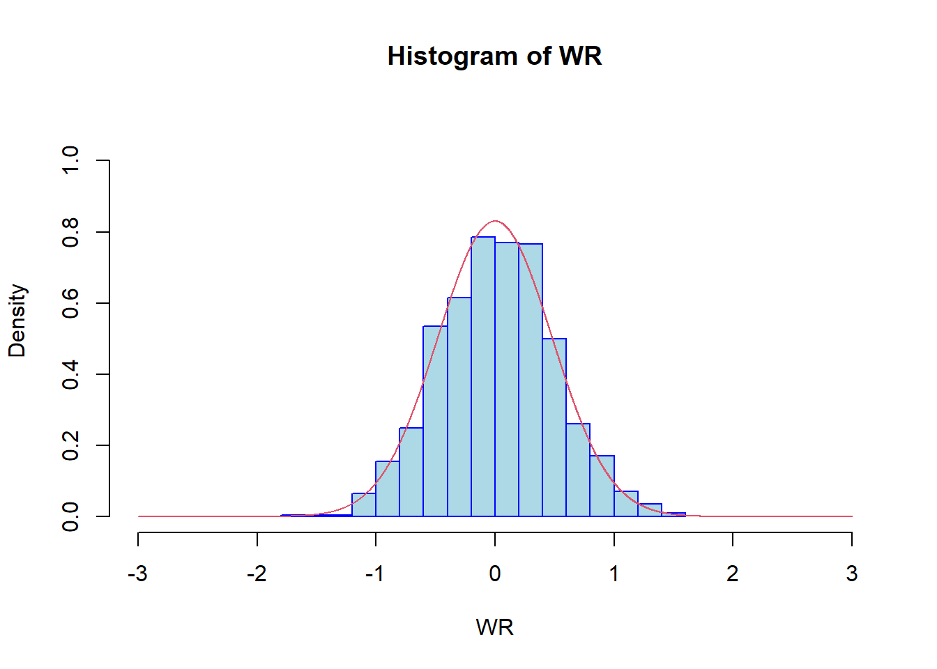

Definition of the win odds

Consider two independent, continuous RVs (random variables) \(\xi\) and \(\eta\). The odds of the win probability is called the win odds of RV \(\eta\) against the RV \(\xi\)

\[\begin{align*} \omega=\frac{P(\eta>\xi)}{P(\eta<\xi)}=\frac{\theta}{1-\theta}. \end{align*}\]

The Mann-Whitney estimate of the win probability can be transformed by the function \(f(x)=\frac{x}{1-x},\ \ x\in(0,1)\) to get an estimate for the win odds. Using the same transformation and the asymptotic normality of the Mann-Whitney estimate it is possible to construct asymptotic confidence intervals for the win odds, for a given asymptotic confidence level.

If \(\omega=1\) then the random variables \(\xi\) and \(\eta\) are stochastically equivalent, while \(\omega>1\) means that \(\eta\) is stochastically greater than (wins against) \(\eta.\) The case \(\omega<1\) means that \(\eta\) loses against \(\xi\). The asymptotic confidence interval of the win odds can be used to test the hypothesis whether \(\omega=1\).

To use the asymptotic normality result described above we need to estimate the asymptotic variance. The package sanon in R allows to estimate the asymptotic standard error of the Mann-Whitney estimate.