Optimality of Estimators in Regular Models
Consistent Estimators
In the estimation problem of a one-dimensional parameter \(\theta\) from an i.i.d. sample \[X^n=(X_1,\cdots,X_n),\ \ X_i\sim F(x,\theta),\,\theta\in\Theta\subset R\] we introduced the notion of consistency of an estimator.This means that whatever the unknown value of \(\theta\) is, this estimator is going to be close to that value in higher probability as \(n\) increases \[\hat\theta_n\approx\theta, \text{ for large } n.\] Now our goal is to quantify this closeness.
Asymptotically Normal Estimators
We say that the estimator \(\hat\theta_n\) is asymptotically normal if \[\frac{\hat\theta_n-\theta}{\sqrt{Var(\hat\theta_n)}}\stackrel{d}{\rightarrow}N (0,1),\] which means that \[P\left(\frac{\hat\theta_n-\theta}{\sqrt{Var(\hat\theta_n)}}<x\right)\rightarrow P(\xi<x),\,x\in R,\,\xi\sim N(0,1).\]
Asymptotically Normal Estimators (Example 1)
Suppose that
\[X^n=(X_1,\cdots,X_n),\ \ X_i\sim N(\theta,\sigma^2),\,\theta\in R,\,\sigma>0.\] We know that the estimator \(\hat\theta_n=\bar X_n=\frac{1}{n}\sum_{i=1}^nX_i\) is an unbiased, consistent estimator for \(\theta.\) By central limit theorem, as \(n\rightarrow+\infty,\) \[\sqrt{n}\frac{\bar X_n-\theta}{\sigma}\stackrel{d}{\rightarrow}N(0,1),\] hence this estimator is also asymptotically normal. The convergence above can be written as (when \(n\rightarrow+\infty\))
\[\sqrt{n}(\bar X_n-\theta)\stackrel{d}{\rightarrow}N(0,\sigma^2).\] Here \(\sqrt{n}\) is rate of convergence of the estimator and \(\sigma^2\) is the asymptotic variance. Hence, higher the rate of convergence or smaller the asymptotic variance, better is the estimator.
Method of Moments
Consider again the estimation problem of a one-dimensional parameter \(\theta\) from an i.i.d. sample \[X^n=(X_1,\cdots,X_n),\ \ X_i\sim F(x,\theta),\,\theta\in\Theta\subset R.\] The idea of the method of moments is based on the fact that we can estimate the mathematical expectation, that is, for any given function \(g(\cdot),\) so that \(E|g(X_1)|<+\infty,\) the following convergence is true \[\begin{align*} \frac{1}{n}\sum_{j=1}^n g(X_j)\stackrel{P}{\rightarrow} E g(X_1). \end{align*}\] Hence, for the estimation of the parameter \(\theta,\) for some \(g(\cdot)\) we can calculate \(E_\theta g(X_1)=T(\theta).\) That will ensure the convergence \[ \frac{1}{n}\sum_{j=1}^n g(X_j)\stackrel{P}{\rightarrow}T(\theta). \]
Method of Moments (Page 2)
Therefore, if the function \(T(\cdot)\) has continuous inverse function \(h=T^{-1},\) then \(\hat\theta_n\) will be a consistent estimator \[\hat\theta_n=h\left(\frac{1}{n}\sum_{j=1}^n g(X_j)\right)\stackrel{P}{\rightarrow}\theta.\] Furthermore, if the function \(h(\cdot)\) is also differentiable and \(E_\theta g^2(X_1)<+\infty,\) then the delta method ensures that the MM estimator is also asymptotically normal \[\sqrt{n}(\hat\theta_n-\theta)\stackrel{d}{\rightarrow}N\left(0,[h'(E_\theta(X_1))]^2 Var_\theta(g(X_1))\right).\]
Method of Moments (Example 2)
Consider the problem of parameter estimation in uniform distribution
\[X_1,\cdots,X_n,\ \ X_i\sim U[0,\theta],\,\theta>0.\] Construct MM estimators using the functions \(g(x)=x,\ \ g(x)=x^2.\)
For \(g(x)=x\) we have \(E_\theta X_1=\frac{\theta}{2}=t,\) were the last equality is a notation. Then, \(\theta=2t=h(t),\) again, the last equality is a notation and \[\frac{1}{n}\sum_{i=1}^n X_i\stackrel{P_\theta}{\rightarrow}E_\theta X_1=t.\] Therefore, \[\hat\theta_n^1=\frac{2}{n}\sum_{i=1}^n X_i\stackrel{P_\theta}{\rightarrow}2t=\theta,\] and \[\sqrt{n}(\hat\theta_n^1-\theta)\stackrel{d}{\rightarrow}N\left(0,\frac{\theta^2}{3}\right).\]
Method of Moments (Example 2, Page 2)
For \(g(x)=x^2\) we have \(E_\theta X_1^2=\frac{\theta^2}{3}=t,\) were the last equality is a notation. Then, \(\theta=\sqrt{3t}=h(t), \ \ (\theta>0)\) again, the last equality is a notation and \[\frac{1}{n}\sum_{i=1}^n X_i^2\stackrel{P_\theta}{\rightarrow}E_\theta X_1^2=t.\] Therefore, \[\hat\theta_n^2=\sqrt{\frac{3}{n}\sum_{i=1}^n X_i^2}\stackrel{P_\theta}{\rightarrow}\sqrt{3t}=\theta,\] and \[\sqrt{n}(\hat\theta_n^2-\theta)\stackrel{d}{\rightarrow}N\left(0,\frac{\theta^2}{5}\right).\]
Method of Moments (Example 2, Page 3)
Hence, in the estimation problem of a one-dimensional parameter \(\theta\) from a uniform distribution
\[X_1,\cdots,X_n,\ \ X_i\sim U[0,\theta],\,\theta>0,\] we have constructed two estimators using the MM \[\hat\theta_n^1=\frac{2}{n}\sum_{i=1}^n X_i, \ \ \hat\theta_n^2=\sqrt{\frac{3}{n}\sum_{i=1}^n X_i^2},\] with the following properties \[ \sqrt{n}(\hat\theta_n^1-\theta)\stackrel{d}{\rightarrow}N\left(0,\frac{\theta^2}{3}\right), \ \ \sqrt{n}(\hat\theta_n^2-\theta)\stackrel{d}{\rightarrow}N\left(0,\frac{\theta^2}{5}\right).\]
Both have the same rate of convergence, but the second one has smaller asymptotic variance, so, asymptotically, the second one is better, although the first one is computationally easier to implement (an important trade-off in Statistics).
Method of Moments (Page 2)
Therefore, if the function \(T(\cdot)\) has continuous inverse function \(h=T^{-1},\) then \(\hat\theta_n\) will be a consistent estimator \[\hat\theta_n=h\left(\frac{1}{n}\sum_{j=1}^n g(X_j)\right)\stackrel{P}{\rightarrow}\theta.\] Furthermore, if the function \(h(\cdot)\) is also differentiable and \(E_\theta g^2(X_1)<+\infty,\) then the delta method ensures that the MM estimator is also asymptotically normal \[\sqrt{n}(\hat\theta_n-\theta)\stackrel{d}{\rightarrow}N\left(0,[h'(E_\theta(X_1))]^2Var_\theta(g(X_1))\right).\]
Method of Moments (Example 2)
Consider the problem of parameter estimation in uniform distribution
\[X_1,\cdots,X_n,\ \ X_i\sim U[0,\theta],\,\theta>0.\] Construct MM estimators using the functions \(g(x)=x,\ \ g(x)=x^2.\)
For \(g(x)=x\) we have \(E_\theta X_1=\frac{\theta}{2}=t,\) were the last equality is a notation. Then, \(\theta=2t=h(t),\) again, the last equality is a notation and \[\frac{1}{n}\sum_{i=1}^n X_i\stackrel{P_\theta}{\rightarrow}E_\theta X_1=t.\] Therefore, \[\hat\theta_n^1=\frac{2}{n}\sum_{i=1}^n X_i\stackrel{P_\theta}{\rightarrow}2t=\theta,\] and \[\sqrt{n}(\hat\theta_n^1-\theta)\stackrel{d}{\rightarrow}N\left(0,\frac{\theta^2}{3}\right).\]
Method of Moments (Example 2, Page 2)
For \(g(x)=x^2\) we have \(E_\theta X_1^2=\frac{\theta^2}{3}=t,\) were the last equality is a notation. Then, \(\theta=\sqrt{3t}=h(t), \ \ (\theta>0)\) again, the last equality is a notation and \[\frac{1}{n}\sum_{i=1}^n X_i^2\stackrel{P_\theta}{\rightarrow}E_\theta X_1^2=t.\] Therefore, \[\hat\theta_n^2=\sqrt{\frac{3}{n}\sum_{i=1}^n X_i^2}\stackrel{P_\theta}{\rightarrow}\sqrt{3t}=\theta,\] and \[\sqrt{n}(\hat\theta_n^2-\theta)\stackrel{d}{\rightarrow}N\left(0,\frac{\theta^2}{5}\right).\]
Method of Moments (Example 2, Page 3)
Hence, in the estimation problem of a one-dimensional parameter \(\theta\) from a uniform distribution
\[X_1,\cdots,X_n,\ \ X_i\sim U[0,\theta],\,\theta>0,\] we have constructed two estimators using the MM \[\hat\theta_n^1=\frac{2}{n}\sum_{i=1}^n X_i, \ \ \hat\theta_n^2=\sqrt{\frac{3}{n}\sum_{i=1}^n X_i^2},\] with the following properties \[ \sqrt{n}(\hat\theta_n^1-\theta)\stackrel{d}{\rightarrow}N\left(0,\frac{\theta^2}{3}\right), \ \ \sqrt{n}(\hat\theta_n^2-\theta)\stackrel{d}{\rightarrow}N\left(0,\frac{\theta^2}{5}\right).\] Both have the same rate of convergence, but the second one has smaller asymptotic variance, so, asymptotically, the second one is better, although the first one is computationally easier to implement (an important trade-off in Statistics).
The Maximum Likelihood Estimator
Consider again the estimation problem of a one-dimensional parameter \(\theta\) from an i.i.d. sample \[X^n=(X_1,\cdots,X_n),\ \ X_i\sim F(x,\theta),\,\theta\in\Theta\subset R.\]
The second method to construct estimators is the Maximum Likelihood Estimator. Here we need the existence of the density functions \(\{f(x,\theta,\,\theta\in\Theta)\}.\) The following function is called the Likelihood function of the above model
\[L(X^n,\theta)=\prod_{i=1}^n f(X_i,\theta).\]
The Maximum Likelihood Estimator (the MLE) is defined as the point of maximum of the likelihood function \[\hat\theta_n^{MLE}=\arg\max_{\theta\in\Theta}L(X^n,\theta).\]
Regular Models
We call the model \(\{f(x,\theta),\,\theta\in\Theta\}\) a regular if the derivative of the density functions \(f(\cdot,\theta)\) exists with respect to \(\theta.\)
Beware that there are other technical conditions as well in the definition of regular models, but we will check only the condition above.
Example The uniform distribution has the density function \[f(x,\theta)=\frac{1}{\theta}I_{[0,\theta]}(x)=\frac{1}{\theta}I_{[0,+\infty)}(x)I_{[x,+\infty)}(\theta).\] This function is not differentiable w.r.t. the unknown parameter \(\theta,\) hence this is not a regular model.
The Properties of the MLE
- Since the natural logarithm is an increasing function, then we can define (if \(f(x,\theta)>0,\,(x,\theta)\in\Theta\times R\)) \[V(X^n,\theta)=\ln L(X^n,\theta)=\sum_{i=1}^n\ln f(X_i,\theta)\] and for the MLE we will have \[\hat\theta_n^{MLE}=\arg\max_{\theta\in\Theta}V(X^n,\theta)=\arg\max_{\theta\in\Theta}\sum_{i=1}^n\ln f(X_i,\theta).\]
The Properties of the MLE (Page 2)
In the regular models the MLE is consistent and asymptotically normal with the asymptotic variance equal to the inverse of the Fisher information \(I^{-1}(\theta)\) \[\sqrt{n}(\hat\theta_n^{MLE}-\theta)\stackrel{d}{\rightarrow}N(0,I^{-1}(\theta)),\] where the Fisher information is defined as \[I(\theta)=\int_{R}\left[\frac{\partial(\ln f(x,\theta))}{\partial\theta}\right]^2f(x,\theta){\rm d} x.\]
If the second derivative of the density functions \(f(x,\theta)\) with respect to \(\theta\) exists then the Fisher information can be calculated by the following formula
\[I(\theta)=-\int_{R}\left[\frac{\partial^2(\ln f(x,\theta))}{\partial\theta^2}\right]f(x,\theta){\rm d} x.\]
An Example of a Non-Regular Model
Consider again the problem of parameter estimation in uniform distribution \[X_1,\cdots,X_n,\ \ X_i\sim U[0,\theta],\,\theta>0.\] The density function of the uniform distribution is given by the formula \[f(x,\theta)=\frac{1}{\theta}I_{[0,\theta]}(x),\] hence the likelihood function will be \[\begin{align*} L(X^n,\theta)&=\frac{1}{\theta^n}\prod_{i=1}^n I_{[0,\theta]}(X_i)=\frac{1}{\theta^n}I_{[0,+\infty)}(X_{(1)})I_{[0,\theta]}(X_{(n)})=\\ &=\frac{1}{\theta^n}I_{[0,+\infty)}(X_{(1)})I_{[X_{(n)},+\infty)}(\theta)\stackrel{a.s.}{=}\frac{1}{\theta^n}I_{[X_{(n)},+\infty)}(\theta), \end{align*}\] which attains its maximum at the point \(\hat\theta_n^\ast=X_{(n)},\) so that is the MLE.
An Example of a Non-Regular Model (Page 2)
Calculate the distribution function of this estimator \[\begin{align*} P(X_{(n)}< x)&=P(\max\{X_1,\cdots,X_n\}<x)=P(X_1<x,\cdots,X_n<x)=\\ &=P(X_1<x)\cdots P(X_n<x)=F^n(x), \end{align*}\] hence \[P(n(\theta-X_{(n)})<x)=P\left(\theta-\frac{x}{n}<X_{(n)}\right)=1-F^n\left(\theta-\frac{x}{n}\right),\] therefore, \(P(n(\theta-X_{(n)})<x)=0,\) for \(x\leq0,\) and for \(x>0\) \[\begin{align*} &P(n(\theta-X_{(n)})<x)=P\left(\theta-\frac{x}{n}<X_{(n)}\right)=1-F^n\left(\theta-\frac{x}{n}\right)=\\ &=1-\left(\frac{\theta-\frac{x}{n}}{\theta}\right)^n=1-\left[\left(1-\frac{x}{\theta n}\right)^{-\frac{n\theta}{x}}\right]^{-\frac{x}{\theta}}\rightarrow1-e^{-\frac{x}{\theta}}. \end{align*}\]
An Example of a Non-Regular Model (Page 3)
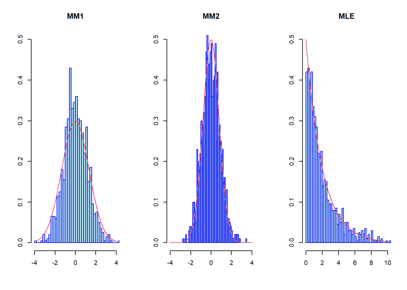
So, for the MLE we have the following convergence to the exponential distribution \[n(\theta-\hat\theta_n^\ast)\stackrel{d}{\rightarrow}E\left(\frac{1}{\theta}\right),\] which means that the rate of convergence for the MLE is \(n,\) unlike the two previous estimators constructed by the method of moments for which the rate of convergence was \(\sqrt{n}.\) In fact, we can show that even non-asymptotically
\[\begin{align*} E_\theta(\hat\theta^\ast_n-\theta)^2=\frac{2\theta^2}{(n+1)(n+2)}<\frac{\theta^2}{3n}=E_\theta(\hat\theta^{1}_n-\theta)^2,\,n>2, \end{align*}\] where \(\hat\theta^1_n=2\bar X_n,\) which entails that even for small sample sizes the MLE is better.
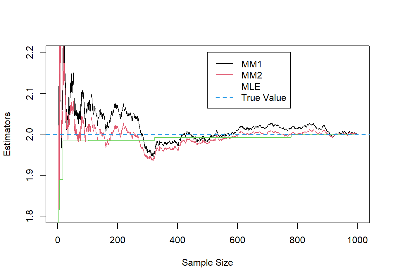
An Example of a Non-Regular Model (Page 4, Simulations)
set.seed(1)
n<-1000
theta<-2
X<-runif(n,0,theta)
th1<-2*cumsum(X)/(1:n)
th2<-sqrt(3*cumsum(X^2)/(1:n))
th<-numeric()
for(i in 1:n){
  th[i]<-max(X[1:i])
}
plot(1:n,th1,type="l",col=1,ylim=c(1.8,2.2),
     xlab="Sample Size",ylab="Estimators")
lines(1:n,th2,type="l",col=2)
lines(1:n,th,type="l",col=3)
abline(h=theta,col=4,lty=2)
legend(500,2.2,col=c(1,2,3,4),lty=c(1,1,1,2),
       legend=c("MM1","MM2","MLE","True Value"))
An Example of a Non-Regular Model (Page 5)
An Example of a Non-Regular Model (Page 6)
n<-10000
m<-1000
theta<-2

th1<-numeric()
th2<-numeric()
th<-numeric()

for(i in 1:m){set.seed(i);X<-runif(n,0,theta)
  th1[i] <- 2*mean(X)
  th2[i] <- sqrt(3*mean(X^2))
  th[i] <- max(X)
}
An Example of a Non-Regular Model (Page 7)
par(mfrow=c(1,3))
x<-seq(-4,4,0.001)
hist(sqrt(n)*(th1-theta),nclass=50,freq=FALSE,
     col="lightblue", border="blue",ylab="",
     xlab="",main="MM1",xlim=c(-4,4),ylim=c(0,0.5))
lines(x,dnorm(x,0,theta^2/3),col=2)

hist(sqrt(n)*(th2-theta),nclass=50,freq=FALSE,
     col="lightblue", border="blue",ylab="",
     xlab="",main="MM2",xlim=c(-4,4),ylim=c(0,0.5))
lines(x,dnorm(x,0,theta^2/5),col=2)

x<-seq(0,10,0.001)
hist(n*(theta-th),nclass=50,freq=FALSE,col="lightblue",
     border="blue",ylab="",xlab="",main="MLE",
     xlim=c(0,10),ylim=c(0,0.5))
lines(x,dexp(x,1/theta),col=2)
An Example of a Non-Regular Model (Page 7)